This repository contains Mathematica implementations of fundamental Image Processing algorithms, developed and explained across multiple laboratory exercises. Each lab explores core techniques such as thresholding, filtering, morphological operations, and frequency-domain image restoration — all implemented from first principles.
Variable Thresholding
Variable Thresholding This lab implements adaptive thresholding to handle uneven illumination in grayscale images. Instead of one global threshold, the image is divided into smaller partitions, and each part gets its own local Otsu threshold. Result: Local thresholds adapt to illumination, correctly separating dark circular objects from the background much better than global thresholding.
Image Restoration
Blurring Function and Restoration Simulates linear motion blur and performs restoration in the frequency domain. Simulates sequential horizontal and vertical motion blurs (T₁, T₂). Restores blurred images by dividing Fourier-transformed images with known H(u, v). Observation:
Effective restoration achieved when motion parameters (a, b, T) are known and noise is negligible.
Morphological Operation
Morphological Operations Implements connected-component labeling using geodesic dilation:
Invert the binary image to make objects white. Select an unlabeled white pixel as a seed. Perform geodesic dilation constrained by the original mask. Label each connected region iteratively.
Hough Transform
Hough Transform Manual implementation for:
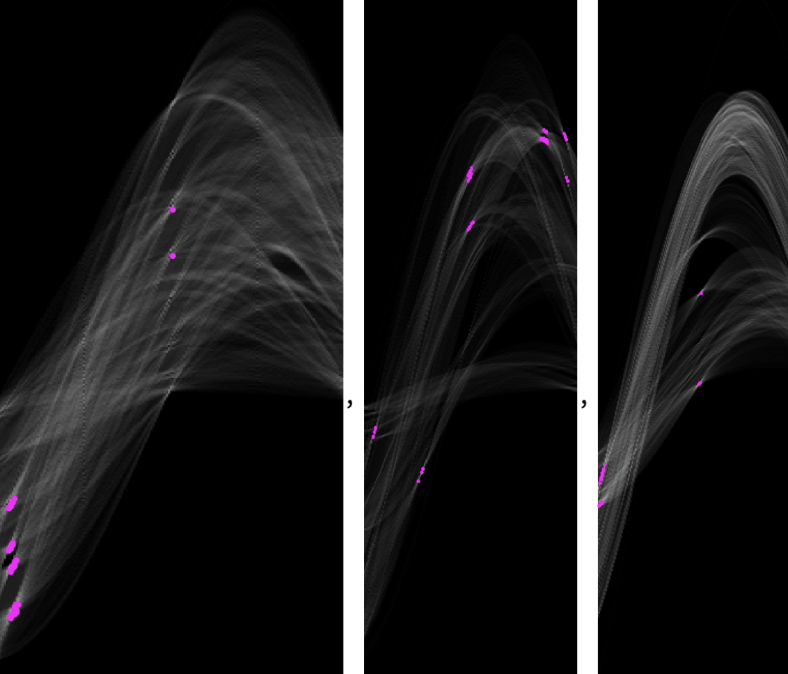
Line detection: Based on Sobel edge maps, ρ–θ parameterization, and local maxima in Hough space.
Circle detection: Uses tangent direction estimation to compute (a, b, r). Result:
Successfully detects multiple lines and circles in complex images such as clocks and coins by iterative voting and duplicate suppression.
Spatial Filtering
Spatial Filtering Implements:
Low-pass filters: Mean and Gaussian
High-pass filters: Laplacian and Laplacian of Gaussian (LoG)
Includes a custom convolution with edge-padding (ConvPadded). Observation:
Mean filter increases blur with kernel size. Gaussian filter maintains more structure. LoG detects sharper edges compared to Laplacian alone.
Histogram Equalization
Histogram Equalization Steps:
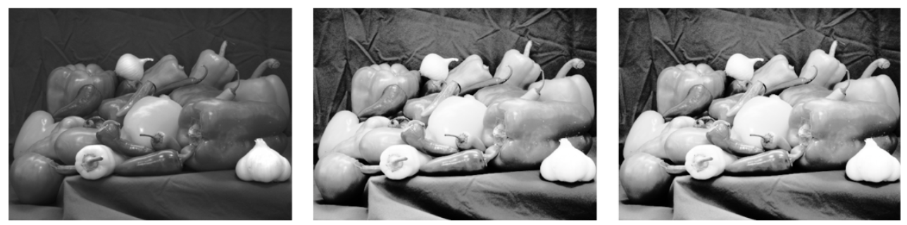
Compute histogram and cumulative distribution function (CDF). Normalize CDF and map it to new intensity values (HistEqualize function). Compare manual results with Mathematica’s HistogramTransform. Result:
Custom implementation produces contrast enhancement nearly identical to the built-in method, with well-distributed intensity levels.
Thresholding
Thresholding Implements two thresholding methods:
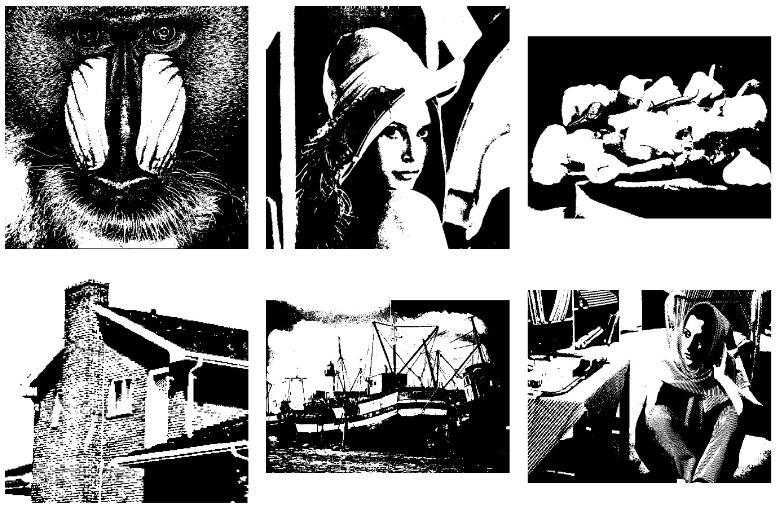
Maximum Normal Line Method: Finds peaks of gray-level histogram and selects threshold by perpendicular distance from the connecting line between peaks. Average Intensities Method: Iteratively updates the threshold based on the mean intensity of pixel groups above and below the threshold until convergence (Δ < 0.01). Result:
Average Intensities Method preserved more image details compared to the first method.